Pulse sequences & the vector model

Use our NMR service for your NMR experiments.

Pulse sequences are used to excite signals that are observed in an NMR spectrometer. They range from general purpose single-pulse experiments to complex highly sophisticated experiments that select specifically interacting nuclei. This page introduces the theory and coventions used to describe pulse sequences.

What you should already know before continuing to read this

Before you start reading about pulse sequences, you should some knowledge of:

• The basis of NMR spectroscopy

If you want to read about this subject first, please go to the link above.

Pulse sequences & the vector model

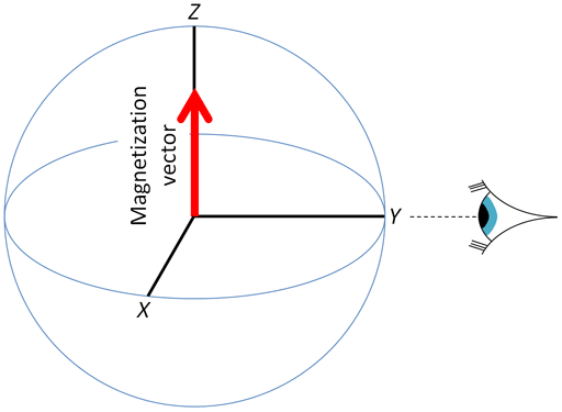
A spinning nucleus, such as a proton, is charged and therefore has a magnetic moment. When it enters an external magnetic field it may either align itself with the field or oppose the field. If the nuclei were in random orientations it would be impossible to observe any net effect. However, it takes energy to oppose the field so slightly fewer nuclei choose to oppose rather than align with the field. This sets up a bulk magnetic moment vector that is the sum of the individual magnetic moments and is the basis of NMR. The overall magnetic moment is called the bulk magnetization of the sample. It is possible to represent the magnetization by a vector in the direction of the magnetic field. The magnetization vector can be shown against coordinates x,y,z with it on the z-axis of a fixed or laboratory frame (fig. 1).

Fig. 1. The laboratory or stationary frame showing the bulk magnetization vector at equilibrium along the z-axis

Larmor precession

Say that we somehow managed to move the magnetization vector by an angle β from the z-axis. (How this is done will be explained later.) In this case the magnetic vector will move around the z-axis describing a cone with the z-axis at its center. The vector's motion has a specific frequency that is representative of it and is called Larmor precession.

If the magnetic field is B₀ then the Larmor precession frequency will be according to equation 1.

Equation 1.

The frequency, ν₀ is the same frequency that will be observed in the NMR spectrum. In the magnet there is a detector (electric coil) that measures the Larmor frequency. The measurement is carried out with a detector in the x,y-plane and when the magnetic vector crosses it during precession it induces a measurable electric current in the coil. The process is similar to the way electric current is generated by a rotating magnet in a coil.

Pulses

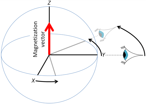
We will now deal with how to move the magnetic vector away from equilibrium. The magnetic field is along the z-axis is the magnetization vector. The vector is moved by transmitting a signal (a radiofrequency signal – rf) from a coil in the detector in the x,y-plane. The problem that we have to deal with is that the induced magnetic field that we have to deal with is much stronger than any electrical signal that can be transmitted through the probe coil of the spectrometer. Instead of using a fixed frame of reference, from here on we use a coordinate framework where the x,y-plane rotates about the z-axis at the observation frequency (usually hundreds of millions of times per second) close to the Larmor precession rate of the material under study (Fig. 2).

Fig. 2. The rotating frame, rotating at or near the Larmor frequency, showing the bulk magnetization vector at equilibrium along the z-axis

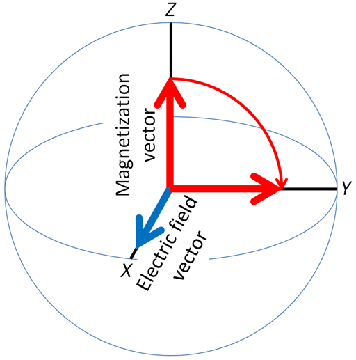
The induced field in on the z-axis becomes proportionate to the rf signal that becomes a fixed electric field vector (E) in the x,y-plane relative on the rotating frame. The correct choice of the rf signal frequency allows the movement of the magnetization vector from the z-axis to the x,y-plane.

The magnetization vector is moved by an angle proportional to the length and intensity of the pulse. If the vector is moved by 90° then the process is called a 90° pulse (fig. 3). It is possible to arrange a 180° pulse so that the magnetization vector goes from +z to –z.

Fig. 3. Effect of a 90°x pulse. The magnetization vector is rotated to the y-axis.

Hard pulse

Most NMR spectroscopic measurements are concerned with measuring more than one signal and each of them has a different Larmor frequency. A sufficiently strong rf pulse is needed to overcome the induced field to move all the signals at different Larmor frequencies away from equilibrium. This is called a hard pulse.

Soft pulse

When the pulse is weaker it is possible to excite a single signal within the spectrum. This is done by choosing a radio frequency identical to the selected signal and reducing its power, thereby reducing the influence of the pulse on other signals. Such pulses are known as selective pulses or soft pulses and may be specially shaped in order to tailor thier excitation profile.

Decoupling

When the signal is split by heteronuclear coupling, for example proton couplings in a carbon spectrum, it is possible to decouple them by continuous irradiation of the coupling nucleus.

Magnetic field gradient pulse

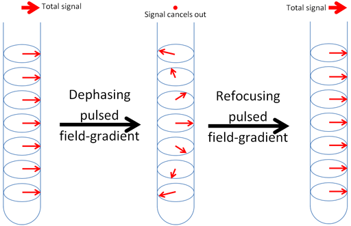
It is possible to apply a magnetic field gradient to the sample. While the field gradient is applied the resonant frequency, which is proportional to the magnetic field, is different in different parts of the NMR tube. If the magnetic field gradient is applied for a short period of time, the phase (direction) of the magnetization will change differently in different parts of the tube such that the overall sum of the magnetization will be zero making the NMR signal disappear. the application of a gradient in the opposite direction allows the signal to be seen again (fig. 4). In combination with rf pulses that act as quantum filters it is possible to observe correlations between nuclei. Likewise, it is possible to measure physical movement in the sample such as diffusion.

Fig. 4. Effect of a magnetic field gradient pulse. The magnetization vector is rotates differently at different positions in the tube cancelling out the total signal. A refocusing gradient pulse can make the total signal reappear depending on its sign and intervening rf pulses.

Acquisition

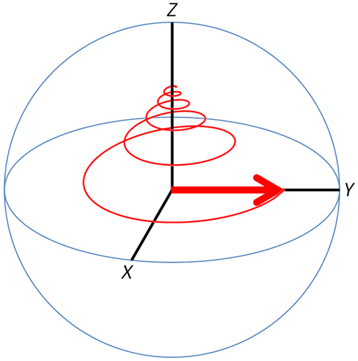
When the magnetization is not at equilibrium, it returns slowly (typically over a period of seconds) to the equilibrium magnetization along the z-axis (fig. 5). In the process, radiofrequency radiation is emitted. This is acquired at the end of the pulse sequence and is called the Free Induction Decay (FID).

Fig. 5. Free induction decay of an excited magnetization vector towards equilibrium in the rotating frame. The magnetization precesses around the z-axis while approaching it.

Symbols used in pulse sequences

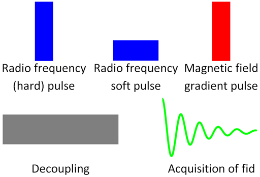
Pulse sequences are represented diagrammatically (fig. 6). Throughout this website, radiofrequency pulses are represented as blue rectangles whose widths represent their duration and whose heights represent their intensity (not to scale). Magnetic field pulses are represented as red rectangles whose heights represent their intensities. Decoupling is represented as a grey rectangle. The free induction decay (FID) is represented as a green decaying sinusoid.

Fig. 6. Symbols used in pulse sequences

A basic pulse sequence

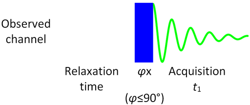
Fig. 7 shows the regular pulse sequence for 1D acquisition using the symbols described above. The sequence starts with a period of time to allow magnetic equilibration known as the relaxation time. There follows a hard radiofrequency pulse that excites the nucleus, transferring the magnetization into the x,y-plane. As the nuclei relax towards equilibrium they emit a radiofrequency signal known as the free induction decay (FID). This sequence relates to only one type of nucleus (such as ¹H) which is the detected in the observed channel in the experiment.

Fig. 7. Basic 1D-NMR pulse sequence

Multi-channel pulse sequences

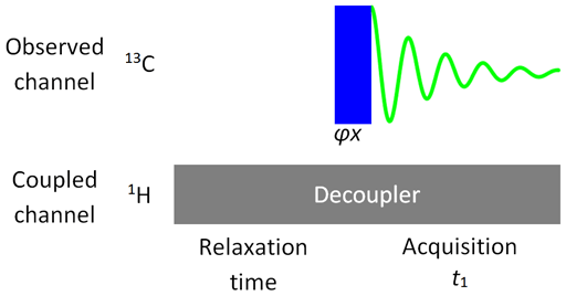
Many experiments involve more than one nucleus and therefore require the use of more than one radiofrequency channel. Note that each of the rf channels are at different frequencies, matched to different nuclei. One of the simplest is the decoupled experiment such as ¹³C decoupled by ¹H. In this experiment (fig. 8), ¹³C is the observed channel and ¹H is the coupled channel (that is decoupled continuously throughout the experiment).

Fig. 8. Decoupling pulse sequence when protons are decoupled from carbons

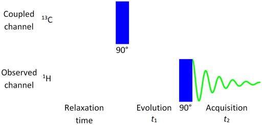
The coupled channel may be used to selectively excite the observed channel in a two-dimensional (2D) experiment. The evolution time, t₁, is the time that is incremented between each row of a 2D acquisition and makes up the extra dimension. In a 2D pulse sequence the symbol for the acquisition time axis is t₂. For example in a simple old-fashioned ¹H-¹³C 2D correlation, the coupled protons are excited and their magnetization allowed to precess for a short period before being used to modulate the carbon signals (fig. 9).

Fig. 9. Basic heteronuclear correlation sequence showing excitation in two channels

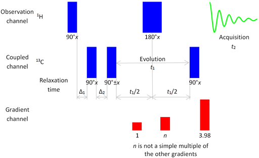
Many modern pulse sequences include a magnetic field gradient channel that is used to selectively refocus signals. For example Fig. 10 shows an example of a three-channel pulse program. In two of the channels, radiofrequency pulses are transmitted and in the third, magnetic gradient pulses are applied. The proton channel is the observed channel while the second channel is that of the ¹³C nucleus coupled to proton. Transmission on all the channels is in parallel. The diagram shows a pulse sequence for a 2D experiment, HMBC that measures proton-carbon correlation.

Under each rf pulse its pulse angle and phase are written. Under the rf channels there is a time-scale (Δ and t₁). The grey lines on the diagram are not usually drawn but have been added here (and only here) for clarity. The relative gradient intensities are shown under the gradient channel. Note that the 180° pulse is drawn wider than the others indicating its longer duration but remember that the times are not drawn to scale. One of the pulse phases is shown as ±x indicating that this sequence is acquired twice and added once with phase +x and once with phase –x.

Fig. 10. Three channel pulse sequence for the 2D HMBC experiment