2D NMR

Use our NMR service for 2D and other NMR experiments.

Types of 2D NMR

Two dimensional (2D) NMR spectroscopy includes:-

Homonuclear

Through bond: COSY, TOCSY, 2D-INADEQUATE, 2D-ADEQUATE
Through space: NOESY, ROESY

Heteronuclear correlation

Examples of 2D spectral assignment

Assignment of 12,14-di^tbutylbenzo[g]chrysene

Assignment of cholesteryl acetate

The basis of 2D NMR

In a 1D-NMR experiment the data acquisition stage takes place right after the pulse sequence. This order is maintained also with complex experiments although a preparation phase is added before the acquisition. However, in a 2D-NMR experiment, the acquisition stage is separated from the excitation stage by intermediate stages called evolution and mixing. The process of evolution continues for a period of time labeled t₁. Data acquisition includes a large number of spectra that are acquired as follows: the first time the value of t₁ is set close to zero and the first spectrum is acquired. The second time, t₁ is increased by Δt and another spectrum is acquired. This process (of incrementing t₁ and acquiring spectra) is repeated until there is enough data for analysis using a 2D Fourier transform. The spectrum is usually represented as a topographic map where one of the axes is f₁ that is the spectrum in the t₁ dimension and the second axis is that which is acquired after the evolution and mixing stages (similar to 1D acquisition). The intensity of the signal is shown by a stronger color the more it is intense.

In the resulting topographic map the signals are a function of two frequencies, f₁ and f₂. It is possible that a signal will appear at one frequency (e.g., 20 Hz) in f₁ and another frequency (e.g., 80 Hz) f₂ that means that the signal's frequency changed during the evolution time. In a 2D-NMR experiment, magnetization transfer is measured. Sometimes this occurs through bonds to the same type of nucleus such as in COSY, TOCSY and INADEQUATE or to another type of nucleus such as in HSQC and HMBC or through space such as in NOESY and ROESY.

The various 2D-NMR techniques are useful when 1D-NMR is insufficient such when the signals overlap because their resonant frequencies are very similar. 2D-NMR techniques can save time especially when interested in connectivity between different types of nuclei (e.g., proton and carbon).

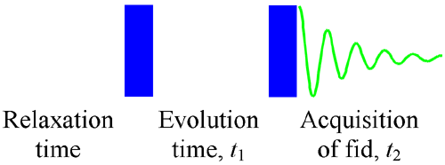
The basic 2D NMR experiment(fig. 1) consists of a pulse sequence that excites the nuclei with two pulses or groups of pulses then receiving the free induction decay (fid). The groups of pulses may be purely radiofrequency (rf) or may include magnetic gradient pulses. The acquisition is carried out many times, incrementing the delay (evolution time - t₁) between the two pulse groups. The evolution time is labeled t₁ and the acquisition time, t₂.

Fig. 1. Basic pulse sequence for 2D acquisition

2D Fourier transform

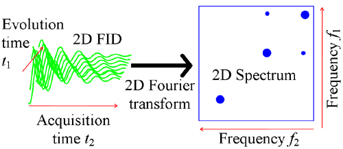
The FID is then Fourier transformed in both directions (fig. 2) to yield the spectrum. The spectrum is conventionally displayed as a contour diagram. The evolution frequency is labeled f₁ and the acquisition frequency is labeled f₂ and plotted from right to left.

Fig. 2. 2D Fourier transform

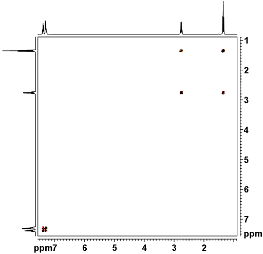
The 2D spectrum is usually plotted with its 1D projections for clarity. These may be genuine projections or the equivalent 1D spectra. In a homonuclear spectrum there is usually a diagonal (with the exception of 2D-INADEQUATE) that represents the correlation of peaks to themselves and is not in itself very informative. The signals away from the diagonal represent correlations between two signals and are used for assignment. For example in the homonuclear COSY spectrum in Fig. 3, the ¹H signal at 1.4 ppm correlates with the ¹H signal at 2.8 ppm because there are cross-peaks but they do not correlate with the signals at 7.3 ppm.

Fig. 3. 2D COSY spectrum of ethylbenzene

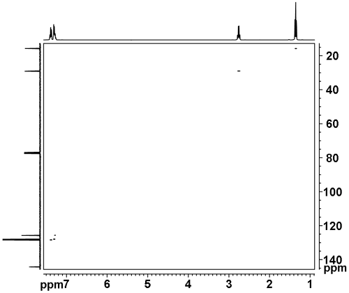
In a heteronuclear spectrum there are no diagonal signals and all the signals represent correlations. For example in the heteronculear HSQC short-range correlation spectrum in fig. 4, the ¹H signal at 1.4 ppm correlates with the ¹³C signal at 15.7 ppm, the ¹H signal at 2.8 ppm correlates with the ¹³C signal at 29.0 ppm, etc.

Fig. 4. 2D HSQC spectrum of ethylbenzene

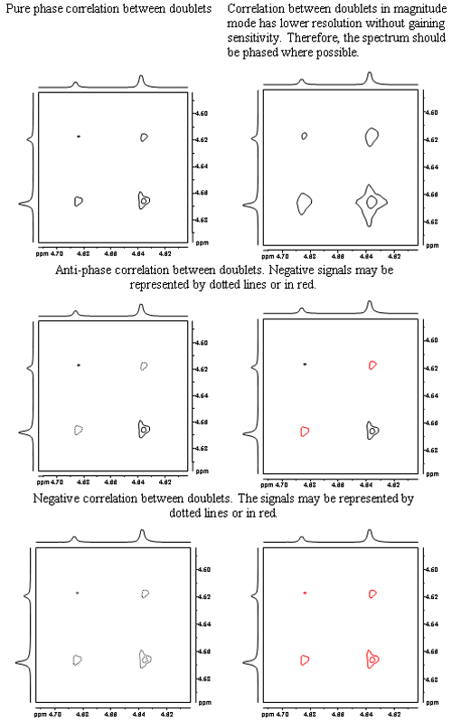
The signals in a 2D spectrum are not always pure phase. Sometimes, the phase cannot be expressed simply as in HMBC and 2D-INADEQUATE, in which case a magnitude spectrum is plotted. However, magnitude spectra sacrifice resolution as compared to pure phase spectra (and unlike window functions that broaden lines, do not yield sensitivity gains). Therefore, wherever possible, the 2D spectrum should be phased. The resulting signals may be pure phase, anti-phase or negatively phased as in the fig. 5. Negative signals are conventionally represented by dotted or red contours.

Fig. 5. Possible phases for a correlation between two doublets